Quant Assignment 2

Part 1:

In trying to decide which cycling team to invest money behind, either Team ASTANA or Team Tobler it is helpful to consider each teams range, mean, median, mode, Kurtosis, Skewness, and Standard Deviation.  Definitions of each of these are below:

• Range: the difference between the highest and the lowest values in a set of data
• Mean: the average or central value of a set of data found by adding all values up and dividing by the total number of values
• Median: the middle or midpoint of a distribution of ranked values 
• Mode: the value that occurs most frequently in a set of data
• Kurtosis: how flat or peaked a curve of data is compared to the normal distribution.      -negative kurtosis (platykurtic): curve is flatter, is a negative number less than -1                  -positive kurtosis (leptokurtic): curve is more peaked, is a positive number greater than 1
• Skewness: measures deviation of symmetry from the mean, can be either positive (longer tail to the right of the line for the mean) or negative (longer tail to the left)
• Standard Deviation: statistical measure of how closely data values are to the mean in a set, a higher standard deviation means the data are spread out farther from the average

The data and calculations for each team are shown below:

Standard Deviation Calculations:

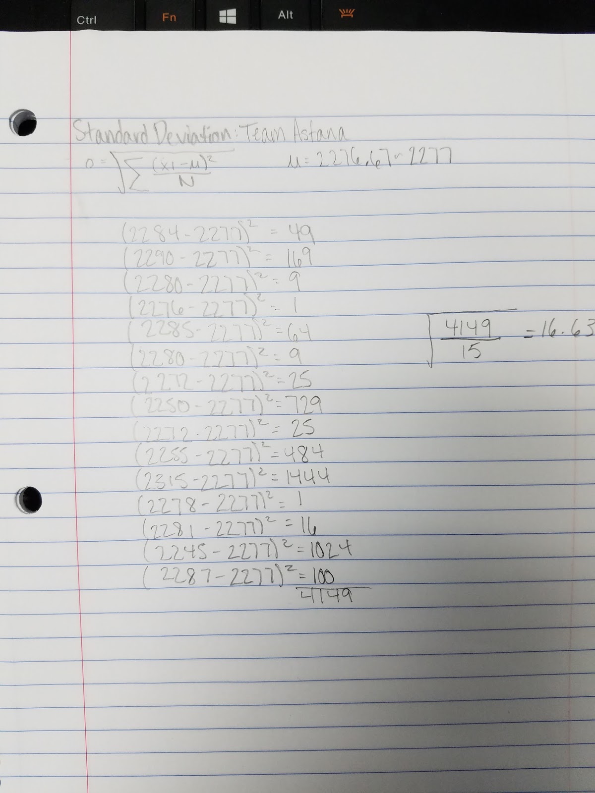
If the entire team that has the better race times gets more money per winning (400,000) and the team owner gets a higher percentage of those winnings (35%) then I would choose Team ASTANA.  Team ASTANA has the lower (fastest) average race time (37 hours and 57 minutes), beating Tobler (38 hours and 5 minutes) by 8 minutes.  The team also has the lowest sum for all its riders 34150 compared to 34282 on team Tobler.  Looking at Kurtosis, team ASTANA is relatively less peaked or close to 0, meaning the data for that team fall closer to the normal distribution.  Team ASTANA is also less skewed than Tobler.  This means that they have data that falls equally to both sides of the mean, indicating that they have riders that are really fast, but also slow.  However, this evens out to give a smaller mean, which means an overall faster team.  The fastest riders are carrying the weight for the team.  A more negative skewness shows that the data leans more to the right and there are relatively few lower numbers, which is what we don't want since low numbers means a faster score.  Lastly, although team ASTANA has a higher standard deviation, meaning it has numbers that fall farther from the mean, its fastest riders are causing the mean to be smaller.  It has riders that deviate more in each direction, which is also showed in the range, but generally it evens out to be a faster team.  Looking at the mean is the bests statistic to support Team ASTANA. 

Part 2:

For this part, population data for Wisconsin Counties was used to find the Geographic Mean Center and the weighted mean center for population in the years 2000 and 2015.  Geographic mean center finds the center of concentration of features using x and y coordinates.  The weighted mean center adjusts for the frequencies of data that are grouped together.  The map produced is shown below:

From the map, it can be seen that the geographic mean center at the county level is located almost exactly in the middle in the state in Wood County.  This is the central tendency, or the average of the x and y coordinates are located at this position.  After weighting the mean center with population data from 2000 and 2015, the mean center moved slightly to the south east to Green Lake County.  Taking the frequency of population into consideration changed the location.  Between the years 2000 and 2015 the mean center shifted very slightly to the west but is still found in the same county, Green Lake.  This could indicate that the population of counties to the west of the coordinate points for the 2000 mean center of population rose in a very small amount, or counties with a higher frequency of greater populations occurred to the west.

Quantitative Methods Assignment 1

Part One:

Nominal Data: this is data that is distinguished by a naming system to label variables.  This data is not usually measurable or quantifiable.  The map below contains nominal data because it uses names to differentiate the distinct climate zones across the globe and the variables do not contain numbers.

Source: http://esdac.jrc.ec.europa.eu/projects/RenewableEnergy/Images/Climate_Zone%2011_s.jpg

Ordinal Data: data that can be put into a ranking order or category based on position on an established scale.  The difference between rank can not be measured.  The map below shows an example of ordinal data because it is ranked into order in three categories with no way measuring the difference between each ranking.

Source: http://aldf.org/wp-content/uploads/2015/12/ALD-127-US-Protection-laws-rankings-map-2015-Large2.png

Interval Data: data that can be measured along a scale with each point being equal distance from one another.  Interval data can not have zero as a starting point and can not be multiplied or divided by.  The map below shows interval data because elevation does not have a starting point and each increment on the map goes up equally.

Source: http://topocreator.com/ned-jpg/city_a/600/mn.jpg

Ratio Data: Data that is measured along a scale with each point being equal distance from one another.  Unlike interval data, ratio data have a known starting point of zero.  The map below shows ratio data because the starting point is zero and progresses by intervals of 8 million.

Source: http://support2.dundas.com/OnlineDocumentation/RSMap/Images/DesigningMaps1.bmp

Part 2
In an effort to visualize where the numbers of female farm operators in Wisconsin are located and where there needs to be an increase in farming among females I have created the following maps.  Each map has a different classification method, therefore changing the look of the map.
The first map, shown below, uses equal interval classification.  Equal interval uses the range of data from highest to lowest and divides that by the number of classes desired, in this case 4.  Each interval will be the same size but might not have the same number of data in them.

Equal Interval

The next map was classified by Jenks Natural Breaks.  Natural Breaks finds the minimum variance in data by finding class breaks based off of differences in size of numbers in a set of data.

Jenks Natural Breaks

The last map is classified using the Quantile method.  This method places an equal amount of units in each class, unlike the equal interval method.

Quantile Method

The company should be targeting counties that are lightest in color, or have the fewest number of female farm operators, since these are the places which would benefit the most for marketing and have the most need to increase their numbers.  The map with the best classification method for the job is the Natural breaks map because it groups similar values the best to give a more accurate representation of the numbers of female farmers in each county.  It also keeps the intervals of classes with fewer female farmers smaller so it is easier to differentiate sizes and target these counties for marketing.  The last class can have a larger grouping because we are not interested in the counties with the highest numbers of female farmers.  From this map it is clear to see that counties in the northern portion make up the largest portion of the state lacking female farmers.